Requirements

• Basic coding experience. Having used python before will help.
• Google account in order to use Google Colab and Google Drive.

What makes a neural network?

We promise to keep things brief and math to a minimum. Let’s take a look at this illustration, then we can go over all of the concepts that are needed for it make sense:

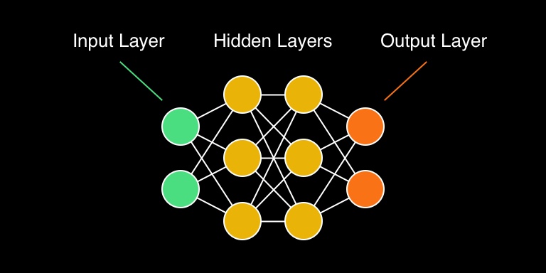
Input Layer

If we go horizontally from left to right, the first column of neurons is called an input layer. As the name suggests, this is where we pass data to the network. The most important concept to understand about the input layer is the shape of the input data.

For example, if we have an input layer of 7 neurons, we must pass a tensor with a shape of (7, 1). Feeding data to the input layer that doesn’t match its shape will usually result in an error.

Explaining tensors is out of scope of this article, so for simplicity let’s just call it a multi-dimensional array, which would look like this:

[23, 81, 43, 83, 1, 66, 41]

Output Layer

The last layer from left to right is called an output layer. We pass data into the input layer and we get the result from the output layer.

For example, in an image classification neural network we would pass an image to the input layer (which would have a shape of (256, 256, 3) for a 256x256 image with 3 color channels) and as an output we get a number from 1 to N, where N is the number of classes that an image could belong to.

Hidden Layers

The layers between the input layer and the output layer are called hidden layers. This is were the magic happens. The process of figuring out what hidden layers to use is the art of machine learning. There are many different ways you can do it and each one has its own advantages depending on what kind or data set your trying to model!

Neurons

Each layer is made of “neurons” and each neuron in a layer is connected to every neuron of the previous and next layer.

And now the final piece to the puzzle - each neuron has a value, which can be expressed as:

Y = ∑(weight * input) + bias

• input - The value of a neuron from the layer on the left.
• weight - Multiplier of how important that value is.
• ∑(…) - The “weighted sum” of the inputs, or the value of each previous neuron, multiplied by the weight of the current neuron, all added together.
• bias - A constant added to the weighted sum. Think of this like a parameter, which the neurons “learn” during the training process.

Finally, the result of Y is passed to an activation function, which modifies Y in a specific way and feeds it to each neuron of the next layer. There are different kinds of activation functions that modify Y in a different way.

Cool! We’re going to stop with the theory here. This is a very simplified explanation of how neural nets work and you’ll have no problem understanding the code that we are about write now. Promise!

Our neural network

Now that we have an idea of what a neural network is, let’s create one and see it in action. Consider those two sets of numbers:

[-1, 0, 1, 2, 3, 4]

[-3, -1, 1, 3, 5, 7]

Do you see a relationship? Here it is:

b = 2 * a - 1

Where a is the input - a number from the top set, and b is the output - the corresponding number from the bottom set. And look at the expression - 2 * a - 1. That looks a lot like the formula weight * input + bias, doesn’t it?

So if we had a neural network with a single neuron and we manage to train it that its weight should be 2 and its bias should be -1, then we would be able to pass any number to it and it would predict a new number that correctly fits the second set of numbers. To illustrate, here is what the neural net would look like:

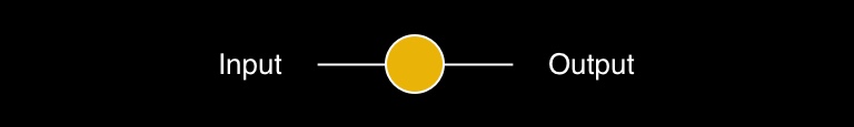
Okay, with the theory and explanations out of the way, let’s write some code!

Frameworks and libraries

With the rise in popularity of machine learning, two frameworks have become leaders TensorFlow and PyTorch. We will use Tensorflow for this tutorial. In addition we’ll import numpy, which is a widely used library among data scientists due to its powerful number crunching capabilities.

Create a new Google Colab notebook and in the first cell import everything that we will need. If you need a quick start guide on Google Colab, check out this excellent guide. Now, back to our code:

import tensorflow as tf
import numpy as np
from tensorflow.keras import Sequential
from tensorflow.keras.layers import Dense

Defining our network

Now for the next cell, let’s create our neural net. First, we define the layers that will make our network. In this case will have a single layer with just one neuron.

layer = Dense(units=1, input_shape=[1])

Dense is one of many helpful classes in TensorFlow. It creates a layer with the given number neurons and an input shape. As we mentioned previously there are many kinds of layers and to keep things simple we’ll leave it at that for now.

Now let’s take that layer and define our neural network:

model = Sequential([layer])

Sequential is another helper class, which in this case takes and array of layers and gives us a model - let’s call it the “template” of our neural net.

Now we tell our neural net how to learn:

model.compile(optimizer='sgd', loss='mean_squared_error')

When we train a neural network it needs to know two things - how close was the prediction to the desired output and how to correct its weights and biases in order to perform better next time.

In order to determine the first, it needs a loss function - in this case mean_squared_error. And for the second, we pass an activation function - sequential gradient descent, or sgd.

The activation and loss functions are what make a network perform the task you want. There is more than one type to choose from, but they all have their importance in determining how well your networks will do at performing certain tasks.

Training

Now we need some data. Our end goal is to give the network a number, and get an output that matches a pattern. In order to train it, we need to pass some inputs and corresponding outputs. Its job will be to figure out the relationship between the two by adjusting its weights and biases (in this case one weight and one bias):

inputs = np.array([-1.0, 0.0, 1.0, 2.0, 3.0, 4.0], dtype=float)
outputs = np.array([-3.0, -1.0, 1.0, 3.0, 5.0, 7.0], dtype=float)

We use numpy to create two arrays containing six float numbers. This is our training data.

This is a good place to execute the code that we wrote so far and make sure it runs without errors.

Now in a new cell we do the actual training:

model.fit(inputs, outputs, epochs=500)

We give the model the inputs and outputs, and tell it to train for 500 cycles, or epochs. Run the cell and you should see something that looks like this:

Epoch 1/500
1/1 [==============================] - 0s 273ms/step - loss: 22.8995
Epoch 2/500
1/1 [==============================] - 0s 3ms/step - loss: 18.2966
...
Epoch 499/500
1/1 [==============================] - 0s 5ms/step - loss: 4.7227e-05
Epoch 500/500
1/1 [==============================] - 0s 6ms/step - loss: 4.6257e-05

Notice how the loss, or the mismatch between the input data and the desired output decreases after each epoch. By the 500th cycle it is 4.6257 to the negative power of 5. This is a very small number, which means our network should be able to make pretty accurate predictions.

Testing our network

print(model.predict([6]))

In the first line we call model.predict() and pass it an array with a shape of (1) - a single dimensional array, or a scalar. It will print the predicted number that should match the pattern between the input and the output data. For example, given the number 6, it should predict 11, because 6 * 2 - 1 = 11

1/1 [==============================] - 0s 108ms/step
[[10.991661]]

Now let’s see how the network learned to do that. Take the layer that we defined previously and print its weights and biases:

print('Here is what I learned: {}'.format(layer.get_weights()))

Here is what I learned: [array([[1.997124]], dtype=float32), array([-0.99108356], dtype=float32)]

The parameters of our single neuron are 1.997124 and -0.99108356. If we replace those in the formula Y = weight \* input + bias, we get:

Y = 1.997124 \* input + (-0.99108356)

And there we go! Our single neuron learned that in order to get from our input data to our desired output, it should multiply the number by 2 and subtract 1 (or close to those numbers anyway).

This is the simplest possible neural network. It’s not very useful, but hopefully it illustrates the most basic concepts of machine learning.

A real-world task that an advanced neural network could perform is instance segmentation. It takes an image, detects objects in it, labels them and draws a mask for each unique object. This is what we use for our product Mouseover - see it in action!

Here is the full code from this tutorial:

import tensorflow as tf
import numpy as np
from tensorflow.keras import Sequential
from tensorflow.keras.layers import Dense

# Create our neural network
layer = Dense(units=1, input_shape=[1])
model = Sequential([layer])
model.compile(optimizer='sgd', loss='mean_squared_error')

# Training data
inputs = np.array([-1.0, 0.0, 1.0, 2.0, 3.0, 4.0], dtype=float)
outputs = np.array([-3.0, -1.0, 1.0, 3.0, 5.0, 7.0], dtype=float)

# Train
model.fit(inputs, outputs, epochs=500)

# Test
print(model.predict([6]))
print('Here is what I learned: {}'.format(layer.get_weights()))

Conclusion

Neural networks are a type of machine learning that have been around for decades, but they’ve become more popular in recent years because of the advances in deep learning and artificial intelligence. In this article, we’ve looked at what neural networks are and how they work. We also created a simple neural network with a single neuron using TensorFlow.

We hope you found this tutorial helpful and informative! If you want to learn more about machine learning or neural networks, follow us on Twitter where we will be publishing more articles on AI and web development, or subscribe to our newsletter. Thanks for reading!

This article has been inspired by the book AI and Machine Learning for Coders by Laurence Moroney. Highly recommended if you are serious about AI and ML!